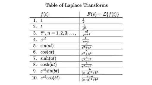
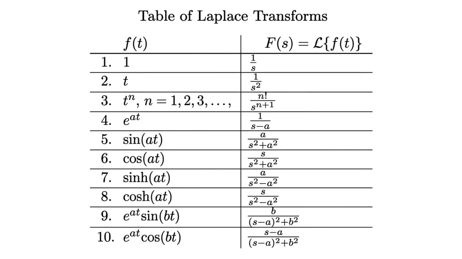
A Laplace table initially appears intimidating, with closely packed rows of symbols and no clear pattern.
Crack the code, though, and it turns into the fastest shortcut in an engineer’s toolkit.
Instead of grinding through differential equations by hand, you look up a match and move on.
Students often memorize a handful of rows, then realize the rest builds naturally from those same properties.
This blog walks through every part of the Laplace transform table, covering pairs, shifting theorems, and step functions, and shows exactly how each fits into solving real problems, step by step, without the guesswork.
Laplace Transform Table at a Glance
The Laplace transform converts functions into a different domain.
It transforms a complex time-based equation into a new language known as the s-domain.
It converts differential equations into algebraic ones, making tough calculus problems solvable with algebra.
Engineers use it to study circuits, control systems, and signals without directly handling derivatives.
The transform works by multiplying a function by an exponential decay term and integrating from zero to infinity.
You do the math in the new language, then translate the answer back to time. That’s the entire secret.
Students utilize this tool in physics and engineering because systems such as springs, circuits, and motors evolve over time. The transform makes it easier to predict their behavior without relying on complex calculus.
Complete Laplace Transform Reference Table
Each function pair on this page is distributed across the separate sections below.
This single table pulls the most-searched pairs into one place, so you can scan it without jumping around the page.
The rightmost column lists the region of convergence, the range of s values where the transform is actually valid, which most quick-reference tables skip.
| f(t) | F(s) | Region of Convergence |
|---|---|---|
| 1 (or u(t)) | 1/s | Re(s) > 0 |
| tn | n!/s(n+1) | Re(s) > 0 |
| eat | 1/(s-a) | Re(s) > a |
| e-at | 1/(s+a) | Re(s) > -a |
| sin(ωt) | ω/(s2+ω2) | Re(s) > 0 |
| cos(ωt) | s/(s2+ω2) | Re(s) > 0 |
| sinh(at) | a/(s2-a2) | Re(s) > |a| |
| cosh(at) | s/(s2-a2) | Re(s) > |a| |
| u(t-a) | e-as/s | Re(s) > 0 |
| δ(t-a) | e-as | All s |
I’m confident in these entries against standard references, but if you’re citing exact convergence conditions in coursework, cross-check them against your textbook’s notation, since some texts define the region strictly and others loosely.
How Do You Read the Table?
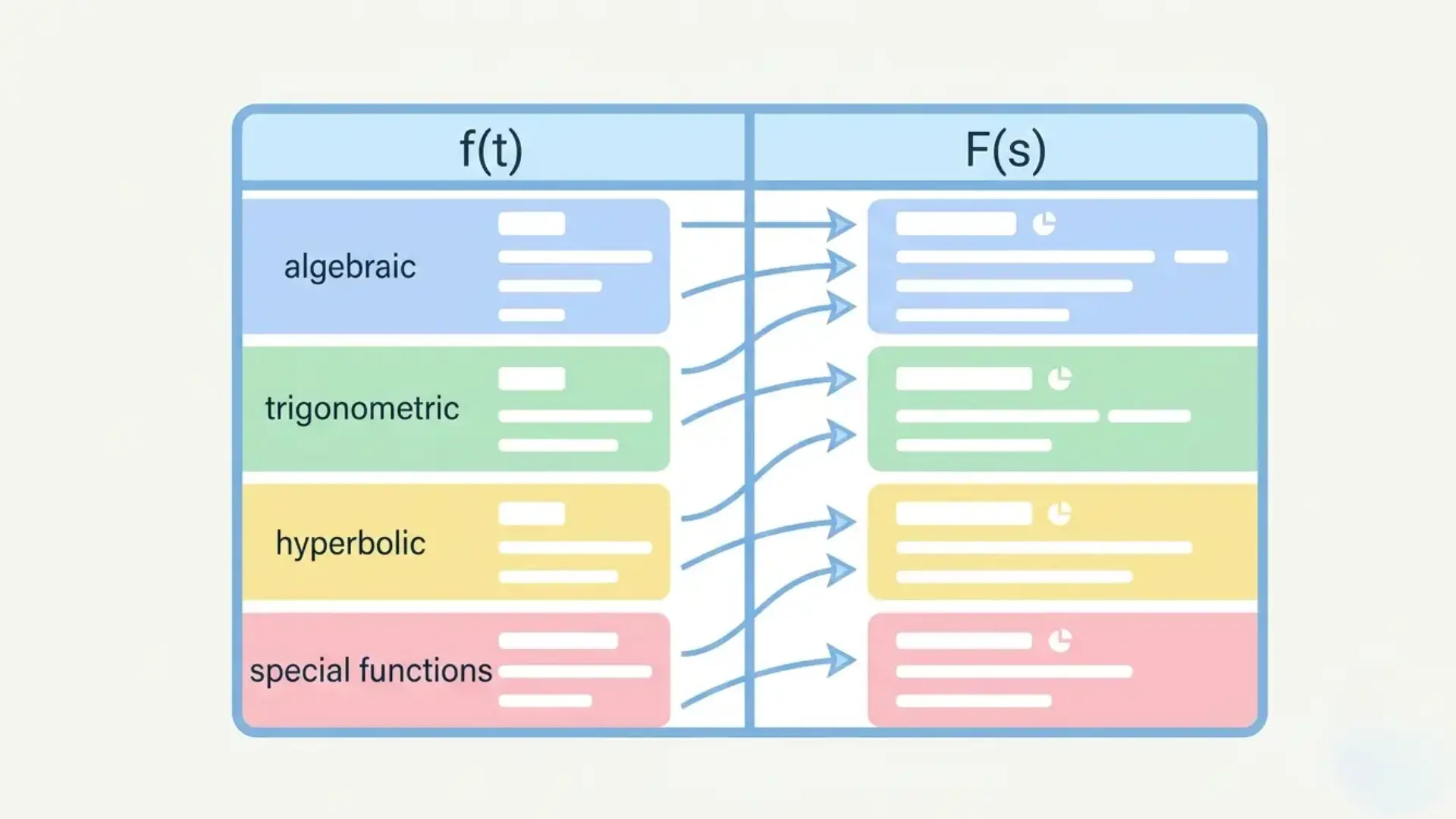
A Laplace transform table works like a dictionary.
One column shows a function of time, f(t). The other shows its matching transform, F(s).
Find your function on the left, then read across to get its s-domain version.
Going backward works too: locate F(s) on the right, and grab the original time function on the left. Most tables group entries by pattern, like exponentials, sine and cosine terms, or step functions.
Match your problem to the closest pattern first.
Constants and coefficients often need slight tweaks to fit a table row, but practice makes this quick.
Basic Laplace Transform Pairs for Common Functions
Some functions repeat regularly, so memorizing their pairs can save time.
- Constant (1): transforms to 1/s
- Exponential (e^at): transforms to 1/(s-a)
- Sine (sin ωt): transforms to ω/(s²+ω²)
- Cosine (cos ωt): transforms to s/(s²+ω²)
- Power function (tⁿ): transforms to n!/(s^(n+1))
- Unit step function (u(t)): transforms to 1/s
Laplace Transforms of Derivatives and Integrals
Derivatives turn into simple algebra once changed. The first derivative of f(t) becomes sF(s) minus f(0).
Higher derivatives follow a similar pattern, adding more initial-condition terms as the order increases.
This is why the method shines with differential equations: no messy chain rules, just multiplication and subtraction.
Integrals work in reverse. Transforming an integral of f(t) gives you F(s) divided by s.
That single division replaces the entire antidifferentiation process. Together, these two rules let you convert an entire differential equation into one algebraic line, ready to solve, then translate back to time.
Laplace Transform Properties You Need for Problem Solving
A few key properties are responsible for most of the work when solving transformation problems.
Master these, and complex expressions will quickly become simple.
1. Linearity
Laplace transforms split sums apart cleanly.
The transform of a sum equals the sum of the transforms, and constants pull straight out front.
This means you can break a complicated function into smaller pieces, transform each piece on its own, then add the results back together. No special tricks needed, just basic algebra.
This feature alone addresses a large portion of textbook questions.
2. Time Shifting
Delaying a function in time multiplies its transform by an exponential term.
If f(t) shifts by a unit, the transform picks up a factor of e^(-as). This shows up constantly in systems with delayed responses, like a switch that flips on a few seconds late.
Recognizing this pattern saves you from having to rework the transform from scratch every time a delay occurs.
3. Frequency Shifting
Multiplying a function by an exponential in time shifts its transform in the s-domain instead.
If f(t) gets multiplied by e^at, the transform F(s) simply shifts to F(s-a).
This mirrors time shifting, just in the opposite direction. It’s especially useful for damped oscillations, where exponential decay pairs with sine or cosine terms.
4. Scaling
Adjusting a function’s time axis by stretching or compressing alters its transform in a predictable way.
Replacing t with at scales both the function and the s-domain variable together.
The transform becomes (1/a)F(s/a). This property matters when comparing systems that run faster or slower versions of the same underlying behavior, without redoing the whole calculation.
5. Convolution
Multiplying two transforms together corresponds to convolving their original functions in time.
This swaps a complicated integral in the time domain for plain multiplication in the s-domain.
Engineers lean on this constantly when analyzing how a system responds to an input signal, since convolution integrals get tedious fast without this shortcut.
6. Initial and Final Value Theorems
These two theorems reveal a function’s behavior at t=0 and as t approaches infinity, directly from F(s).
No inverse transform required. The initial value theorem uses the limit of sF(s) as s approaches infinity. The final value theorem uses the limit as s approaches zero.
Both save time when you only need endpoint behavior, not the full solution.
7. Differentiation in the s-Domain
Multiplying a function by t corresponds to differentiating its transform with respect to s, then flipping the sign.
If f(t) is multiplied by t, the transform becomes -dF(s)/ds.
This property comes in handy for functions like t·sin(ωt) or t· e^ (at), where building the transform from scratch would take far longer than simply taking a derivative.
First Shifting and Second Shifting Theorems
Picture a circuit that switches on late, or a signal that carries a decay factor baked in.
That’s the role these theorems play effectively.
- First Shifting Handles the Decay Case: Multiplying a function by e^at shifts its transform in s.
- Second, Shifting Handles the Delay Case: Hold a function back until t=a, then the transform gains an exponential multiplier.
Together, they cover almost every real-world scenario involving delayed switches or damped signals.
Skip these, and you’re stuck rebuilding transforms manually for every delayed or decaying system you meet.
Common Exponential, Trigonometric, and Hyperbolic Functions
In addition to the basics, these function groups cover most of the problem sets you’ll encounter.
1. Exponential Functions
Exponentials model growth and decay, and their transforms stay simple.
A negative exponent, e^(-at), transforms to 1/(s+a), the mirror image of the growth case.
These functions describe cooling objects, discharging capacitors, and fading signals. Since the transform only flips a sign in the denominator, switching between growth and decay problems takes almost no extra work.
2. Trigonometric Functions
Damped oscillations combine exponentials with sine or cosine, and their transforms shift accordingly.
For e^(-at)sin(ωt), the transform becomes ω/((s+a)²+ω²).
Swap sine for cosine, and the numerator changes to (s+a).
These pairs describe vibrating systems that lose energy over time, like a shock absorber settling after a bump.
3. Hyperbolic Functions
Hyperbolic sine and cosine behave like their trigonometric cousins but without oscillation.
sinh(at) transforms to a/(s²-a²), while cosh(at) transforms to s/(s²-a²). Notice the minus sign instead of a plus; that’s the only real difference from the trig versions.
These show up in problems involving exponential growth curves and certain heat transfer equations
Inverse Laplace Transform Table
Reversing the process involves reading the pairs from right to left, and this table shows the most common ones.
| F(s) | f(t) |
|---|---|
| 1/s² | t |
| 1/(s-a)² | t·e^at |
| s/((s²+ω²)²) | (t/2ω)·sin(ωt) |
| 1/((s-a)(s-b)) | (e^at – e^bt)/(a-b) |
| a/(s(s²+a²)) | 1 – cos(at) |
| 1/(s²+2as+b) | Depends on the discriminant; check for real or complex roots |
Laplace Transforms of Step, Impulse, and Piecewise Functions
Real systems rarely turn on smoothly, so these functions model sudden jumps and jolts.
Unit Step Function
The unit step function jumps from 0 to 1 at a chosen point, modeling a switch flipping on.
Its transform, u(t-a), equals e^(-as)/s. This building block combines with second shifting to describe any function that starts partway through a timeline, like a machine kicking on mid-cycle.
Unit Impulse Function
The unit impulse, or Dirac delta function, represents a sudden spike with zero width and infinite height. Its transform is beautifully simple: L{δ(t-a)} equals e^(-as).
This models instantaneous events, like a hammer strike on a beam or a sudden voltage spike in a circuit.
Piecewise Functions
Piecewise functions change definition across different time intervals, and step functions help stitch them together.
You express each piece using shifted unit steps, then transform the whole thing using second shifting rules.
This approach avoids splitting the integral by hand, turning a multi-part function into one clean expression
How to Use a Laplace Transform Table Step by Step
Using a structured approach makes working with a table much easier.
- Step 1: Provide the specific function you want to modify or reverse.
- Step 2: Divide it into smaller parts by applying linearity, if necessary.
- Step 3: Pair each item with the nearest corresponding table entry.
- Step 4: Modify constants or coefficients to ensure an exact match.
- Step 5: Implement any necessary rules for delays or exponential factors.
- Step 6: Merge the separate results into a single expression.
- Step 7: Verify the final answer aligns with established boundary behavior.
Laplace Transform Table for Differential-Equation Problems
These examples illustrate the full table lookup process, showing which rows and effects are used at each stage.
Example 1: Polynomial-Exponential Combination
Find the Laplace transform of f(t) = t²e^(3t).
This matches the table row for tⁿe^(at) directly, with n = 2 and a = 3.
Applying the formula n!/(s − a)ⁿ⁺¹ gives 2!/(s − 3)³, which simplifies to 2/(s − 3)³.
No properties are needed since the function matches an existing row exactly.
Example 2: Shifted Sinusoid
Find the Laplace transform of f(t) = e^(2t)sin(4t).
This matches the row for e^(at) sin(bt), with a = 2 and b = 4.
Using the formula b/((s − a)² + b²) gives 4/((s − 2)² + 16).
The frequency shifting property is already built into this row, so a single lookup handles the entire function.
Example 3: Solving a First-Order ODE
Solve y’ + 3y = e^(2t), with y(0) = 0.
Taking the Laplace transform of both sides gives sY(s) − y(0) + 3Y(s) = 1/(s − 2).
Substituting y(0) = 0 and solving for Y(s) gives Y(s) = 1/((s − 2)(s + 3)).
Partial fractions split this into 1/5 · [1/(s − 2) − 1/(s + 3)].
Applying the inverse table to each term gives y(t) = 1/5 · (e^(2t) − e^(−3t)).
These entries cover the transforms that appear most often in coursework and applied problems. The properties table below extends this list to functions that don’t match a row directly.
Download the complete Laplace table with practice questions
How to Handle Expressions that Are Not Directly in the Table
Some expressions do not instantly correspond to a table row, but there are methods to bridge this gap.
- Break fractions apart using partial fraction decomposition first.
- Complete the square in the denominator for quadratic terms.
- Factor out constants to expose a recognizable pattern.
- Rewrite polynomials in the numerator using synthetic division.
- Use the convolution theorem for products of two transforms.
- Apply differentiation or integration in the s-domain for tricky multipliers.
When to Use a Table, Algebra, or Partial Fractions
Picking the right tool up front saves time and effort, and this table sorts out which method fits which situation.
| Situation | Best Method |
|---|---|
| Expression matches a standard form | Direct table lookup |
| Multiple terms added together | Algebra with linearity |
| Repeated or irreducible denominator | Partial fractions |
| Product of two separate functions | Convolution theorem |
| Simple constant or coefficient mismatch | Quick algebraic adjustment |
| Complicated rational function overall | Partial fractions, then table |
Common Laplace Table Mistakes and How to Avoid Them
Small mistakes now can lead to major errors later, so check for these regularly.
1. Forgetting Initial Conditions: Derivative transforms include terms like f(0), and skipping them throws off the entire solution. This mistake often occurs under time pressure when algebra feels routine.
Always write out the full derivative rule first, then plug in known conditions.
A missing initial value can make an otherwise correct answer completely wrong.
2. Misreading Table Rows: Rows with similar formulas, like sine and cosine pairs, get swapped easily.
A single misplaced s or ω changes the entire result. Slow down when scanning tables, and double-check which row matches sine versus cosine before copying anything over.
3. Ignoring Region of Convergence: Every transform has a region of convergence, and ignoring it can lead to invalid results in edge cases. Most problems skip this detail, but it’s important for advanced applications.
Note the convergence condition, especially with exponential terms.
4. Skipping Partial Fractions: Complex denominators require partial fraction decomposition before matching a table entry; skipping this wastes time. Always fully simplify first.
5. Mixing Up Shifting Rules: First and second shifting appear similar, and confusing them distorts results. First shifting shifts s when time is exponential; second shifting shifts time and adds an exponential to s.
Swapping them makes the answer wrong. Remember which domain each rule shifts before applying.
End Note!
Working through a Laplace transform table stops feeling like memorization once the properties click into place.
Each row connects to a broader pattern, and spotting that pattern turns lookup into intuition.
Circuits, vibrations, and control systems all lean on the same handful of transforms, applied again and again. Keep this table nearby while solving problems, and cross-check answers whenever something feels off.
Which row on this table do you look up the most?
Drop it in the comments, or ask about a function that didn’t make the list, and we’ll work through it.
Frequently Asked Questions (FAQ’s)
1. What is a Laplace Transform Used for?
It converts differential equations into algebraic ones, simplifying the solution of circuit, control, and signal problems.
2. What is the Laplace Transform of a Constant?
The Laplace transform of a constant, like 1, equals 1/s in the s-domain.
3. How Do You Find the Inverse Laplace Transform?
Match F(s) to a table entry, then read the corresponding f(t) on the time side.
4. What’s the Difference Between Laplace and Fourier Transforms?
Laplace handles transient, unstable signals; Fourier focuses on steady-state, purely oscillatory signals over time.
5. Why Use Partial Fractions in Laplace Transforms?
They break complex rational expressions into simpler pieces that match standard table entries directly.

Dr. Naomi Chen, PhD (Stanford) in Educational Psychology, spent a decade designing evidence-based curricula for K-12 schools. She joined us in 2024 to translate learning science into practical study tactics, classroom tools, and parenting tips. In her spare time, Naomi mentors robotics teams and reviews children’s literature.